Determine subcooling principles and practical applications

Published

determine subcooling
Table of Contents

Subcooling plays a pivotal role in optimizing refrigeration and HVAC systems by enhancing thermal efficiency and reducing energy consumption. This process involves cooling a refrigerant below its saturation temperature to prevent flash gas formation, thereby improving system performance and longevity. Understanding the thermodynamic principles, measurement techniques, and control strategies behind subcooling is essential for engineers and technicians tasked with designing, maintaining, or troubleshooting modern refrigeration cycles.

The effectiveness of subcooling hinges on precise instrumentation, system design, and operational adjustments tailored to specific refrigerants and applications. From commercial air conditioning to industrial chillers, the correct implementation of subcooling can yield measurable energy savings while mitigating risks such as compressor wear and inefficient heat rejection. This discussion explores the fundamentals, measurement methodologies, real-world applications, and advanced control strategies that define subcooling as a cornerstone of high-performance thermal systems.

determine subcooling

Fundamentals of Subcooling in Refrigeration Systems: Thermodynamic Principles and Phase Behavior

Subcooling represents a critical thermodynamic state in refrigeration cycles where the refrigerant remains in a liquid phase below its saturation temperature at a given pressure. This process enhances system efficiency by reducing flash gas formation in the expansion device and improving heat transfer during condensation. The relationship between subcooling, saturation conditions, and refrigerant properties is governed by fundamental laws of thermodynamics, including the Clausius-Clapeyron equation and the principles of phase equilibrium. Understanding these interactions is essential for optimizing refrigeration system performance, particularly in applications requiring precise temperature control, such as commercial refrigeration, air conditioning, and industrial cooling processes.

The thermodynamic behavior of refrigerants during subcooling is best visualized through phase diagrams, which map temperature, pressure, and enthalpy relationships. For common refrigerants like R-134a and R-410A, these diagrams reveal distinct zones where subcooling occurs—typically below the saturated liquid line at constant pressure. The enthalpy-temperature curves further illustrate how subcooling reduces the refrigerant’s internal energy, thereby increasing its cooling capacity and minimizing energy losses in the system.

Thermodynamic Principles Governing Subcooling

Subcooling occurs when a refrigerant liquid is cooled below its saturation temperature at a constant pressure, transitioning from a saturated liquid state to a subcooled liquid state. This process is governed by the following thermodynamic principles:

1. Phase Equilibrium and Saturation Curves
The saturation temperature of a refrigerant at a given pressure is determined by the balance between vapor and liquid phases. For example, at 10 bar for R-134a, the saturation temperature is approximately 39.4°C. Subcooling extends the liquid phase beyond this temperature, reducing the likelihood of vapor formation during pressure drops (e.g., through an expansion valve).

2. Enthalpy and Internal Energy Reduction
Subcooling lowers the refrigerant’s enthalpy (h) without altering its pressure. The specific enthalpy of a subcooled liquid is calculated as:

\( h_{sub} = h_{f} + c_{p,liq} \cdot (T_{sat} - T_{sub}) \)
where \( h_{f} \) is the saturated liquid enthalpy, \( c_{p,liq} \) is the specific heat of the liquid refrigerant, \( T_{sat} \) is the saturation temperature, and \( T_{sub} \) is the subcooling temperature. This reduction in enthalpy directly impacts the system’s coefficient of performance (COP) by decreasing the work required for compression.

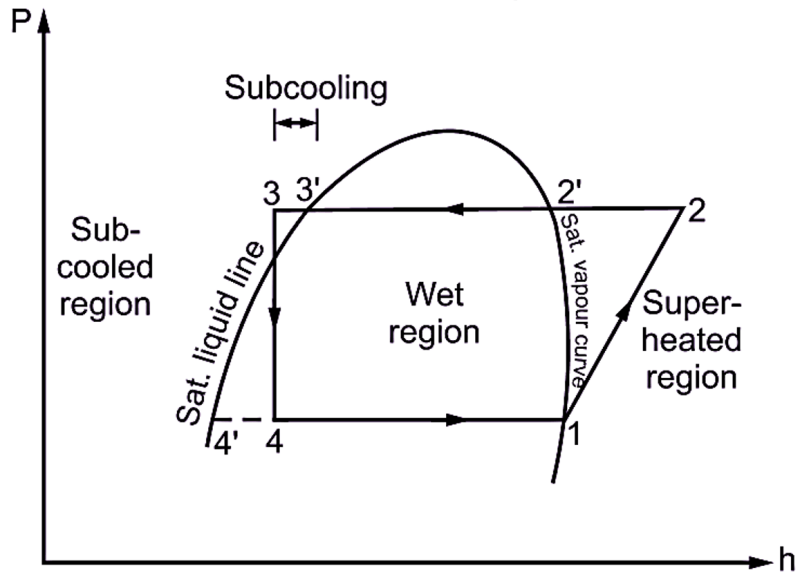
3. Pressure-Enthalpy (P-h) Diagrams and Subcooling Zones
In P-h diagrams, subcooling is represented as a horizontal shift leftward from the saturated liquid line at constant pressure. For instance, in R-410A, subcooling by 5°C at 40 bar reduces the refrigerant’s enthalpy from ~250 kJ/kg (saturated liquid) to ~230 kJ/kg (subcooled liquid). This visualization underscores how subcooling tightens the liquid’s thermodynamic boundaries, enhancing heat rejection efficiency in the condenser.

4. Impact on Latent Heat and Sensible Heat Transfer
Subcooling does not affect the latent heat of vaporization (the energy required to transition from liquid to vapor at saturation). However, it increases the sensible heat transfer capacity of the liquid refrigerant, as additional heat must be removed to further lower its temperature. This is particularly advantageous in systems where condenser exit temperatures must be minimized to prevent compressor floodback or oil dilution.

Phase Diagrams and Subcooling Visualization for Common Refrigerants

Phase diagrams for refrigerants like R-134a and R-410A provide a graphical representation of subcooling zones, illustrating how temperature, pressure, and enthalpy interact. Below are key features of these diagrams relevant to subcooling:

1. Temperature-Entropy (T-s) Diagrams
In T-s diagrams, the saturated liquid line slopes downward from left to right, while the subcooled liquid region lies below this line. For R-134a at 10 bar:

  • The saturated liquid temperature is 39.4°C.
  • Subcooling to 30°C (9°C below saturation) shifts the state point leftward, reducing entropy and enthalpy.
  • The area under the saturated liquid line represents the subcooling potential, which is maximized in high-pressure condensers.

    2. Pressure-Enthalpy (P-h) Diagrams
    P-h diagrams explicitly show subcooling as a horizontal extension from the saturated liquid point. For R-410A at 40 bar:

  • Saturated liquid enthalpy: ~250 kJ/kg at 40°C.
  • Subcooled liquid enthalpy at 35°C: ~240 kJ/kg.
  • The diagram’s curvature highlights that subcooling becomes less efficient at higher pressures due to reduced liquid-specific heat capacity.

    3. Critical Points and Subcooling Limits
    Near the refrigerant’s critical point (e.g., R-134a at 101.1 bar, 101.1°C), subcooling becomes impractical because the liquid and vapor phases converge. Practical subcooling ranges are typically 3–10°C below saturation for most commercial applications.

    Comparison of Refrigerant States: Superheated Vapor, Saturated Liquid, and Subcooled Liquid

    The following table contrasts the thermodynamic properties of superheated vapor, saturated liquid, and subcooled liquid states for R-134a at 10 bar (saturation temperature: 39.4°C). Key metrics include specific volume (\( v \)), enthalpy (\( h \)), and entropy (\( s \)).
    Property Superheated Vapor (e.g., 50°C) Saturated Liquid (39.4°C) Subcooled Liquid (30°C)
    Phase Vapor Liquid-Vapor Equilibrium Liquid Only
    Specific Volume (\( v \), m³/kg) 0.022 0.00089 0.00087
    Enthalpy (\( h \), kJ/kg) 430.0 250.0 230.0
    Entropy (\( s \), kJ/kg·K) 1.72 0.93 0.90
    Heat Transfer Mechanism Sensible heat (superheat) Latent heat (phase change) Sensible heat (subcooling)
    System Impact Reduces compressor work if minimized Critical for evaporator efficiency Prevents flash gas, improves condenser performance
    Key Observations:
  • Superheated vapor has the highest specific volume and enthalpy, requiring more compressor work.
  • Saturated liquid marks the transition point where latent heat absorption begins.
  • Subcooled liquid exhibits the lowest enthalpy and entropy for the given pressure, optimizing heat rejection and reducing expansion losses.
  • Subcooling’s Role in the Vapor-Compression Cycle

    Subcooling directly influences the refrigerant’s heat rejection and absorption processes within the vapor-compression cycle. The following schematic breakdown illustrates these interactions:

    1. Condenser and Subcooling Zone
    In the condenser, the refrigerant transitions from superheated vapor to saturated liquid and then to subcooled liquid. Subcooling ensures that the refrigerant entering the expansion device (e.g., thermostatic expansion valve) remains fully liquid, preventing:

  • Flash gas formation, which reduces cooling capacity.
  • Pressure drops across the expansion valve, improving system efficiency.
  • A well-designed condenser achieves subcooling by extending the heat exchange surface or using secondary refrigerants (e.g., water-cooled condensers).

    2. Expansion Device and Flash Gas Mitigation
    The expansion valve’s primary function is to reduce the refrigerant’s pressure, enabling evaporation in the evaporator. Without subcooling, a portion of the liquid may flash into vapor due to pressure drops, leading to:
  • Reduced evaporator effectiveness.
  • Increased compressor workload to
  • determine subcooling - Ilustrasi 2

    Measurement Techniques and Instrumentation for Subcooling

    Accurate measurement of subcooling is critical for optimizing refrigerant performance, preventing system inefficiencies, and extending equipment lifespan. Instrumentation must account for refrigerant-specific properties, environmental variables, and dynamic operational conditions. This section examines primary measurement tools, calibration procedures, common errors, and the role of software-assisted verification in ensuring precision.

    Primary Instruments for Real-Time Subcooling Measurement

    Subcooling is determined by comparing the refrigerant’s saturated liquid temperature (at a given pressure) to its actual liquid temperature downstream of the condenser. The following instruments are standard in industrial and commercial refrigeration systems:

    - Thermocouples and RTDs (Resistance Temperature Detectors)
    Thermocouples (e.g., Type K, T, or J) are widely used due to their fast response and low cost, with accuracy ranging from ±0.5°C to ±2.5°C depending on calibration. RTDs (e.g., Pt100) offer higher precision (±0.1°C to ±0.5°C) but require stable electrical power. Installation best practices include:

  • Placing sensors 10–15 cm downstream of the condenser outlet to avoid temperature gradients.
  • Ensuring full immersion in the liquid refrigerant to eliminate vapor exposure.
  • Using shielded or armored cables in high-vibration environments (e.g., near compressors).
  • Avoiding proximity to heat sources (e.g., electrical components, sunlight) to prevent false readings.
  • - Pressure Gauges and Transmitters
    Subcooling calculations rely on saturated liquid temperature, derived from refrigerant pressure via pressure-enthalpy (P-h) charts or software. Digital pressure transmitters (e.g., ±0.1% full-scale accuracy) are preferred over analog gauges for dynamic systems. Key considerations:

  • Equilibrium pressure measurement: Ensure the gauge taps are isolated from vapor pockets (e.g., using U-tube traps or sight glasses).
  • Refrigerant compatibility: Use sealed gauges for ammonia (NH₃) or burst discs for flammable refrigerants (e.g., hydrocarbons).
  • Temperature compensation: Some transmitters include PT100 inputs to adjust for ambient temperature effects.
  • - Digital Sensors and Data Loggers
    Modern systems employ smart sensors (e.g., Honeywell ST3000, Siemens SITRANS) with built-in calibration and wireless communication. Features include:

  • Multi-point averaging to reduce noise in pulsating flows.
  • Self-diagnostics for sensor drift or signal loss.
  • Integration with SCADA/PLC systems for real-time monitoring.
  • Calibration Procedures for Refrigerant Temperature Sensors in Closed-Loop Systems

    Sensor calibration ensures subcooling measurements align with thermodynamic principles. A structured approach minimizes errors in closed-loop systems (e.g., chillers, cascade refrigeration):

    Preparation Phase

  • Environmental Controls: Conduct calibration in a temperature-stabilized chamber (e.g., ±0.5°C variation) with humidity <60% to prevent condensation on sensor surfaces.
  • Refrigerant Charge Verification: Use a coremeter or mass flow sensor to confirm the system is at design charge levels (overcharging can mask subcooling errors).
  • Static Pressure Stabilization: Allow the system to operate at steady-state for ≥30 minutes before calibration to eliminate transient pressure fluctuations.
  • Step-by-Step Calibration Process
    1. Reference Point Establishment

  • Immerse the sensor in a reference fluid (e.g., distilled water or silicone oil) with a certified thermometer (traceable to NIST/ISO standards).
  • For refrigerant-specific calibration, use a pressure-controlled test cell (e.g., ASHRAE Standard 41.8 compliant) filled with the target refrigerant (e.g., R-134a, R-410A).
  • Record the saturated liquid temperature at known pressures (e.g., 10 bar, 20 bar) using NIST REFPROP or manufacturer-provided tables.
  • 2. Sensor Immersion and Data Acquisition

  • Submerge the sensor fully in the liquid phase, ensuring no air bubbles are trapped.
  • Log temperature and pressure simultaneously using a data logger (e.g., Fluke 289, Agilent 34970A) with a sampling rate of ≥1 Hz.
  • Repeat measurements at three pressure points to account for nonlinearities in refrigerant properties.
  • 3. Error Correction and Adjustment

  • Compare sensor readings to reference values and calculate systematic bias (e.g., +0.8°C offset).
  • Adjust calibration constants via sensor firmware (for digital sensors) or manual offset correction (for analog systems).
  • Validate adjustments by recirculating the refrigerant through the condenser and verifying subcooling against psychrometric charts.
  • Post-Calibration Verification

  • Field Testing: Deploy calibrated sensors in the system and cross-check with secondary instruments (e.g., a portable Testo 440 refrigerant analyzer).
  • Documentation: Record calibration dates, reference standards, and uncertainty budgets (e.g., ±0.3°C total uncertainty).
  • Common Errors in Subcooling Measurement and Troubleshooting

    Incorrect subcooling readings often stem from sensor placement, environmental factors, or system dynamics. Below is a responsive table outlining frequent issues and corrective actions:
    Error Source Troubleshooting Steps
    Sensor Lag

    - Slow response in pulsating flows (e.g., near compressor discharge).

    - Common in thermowells with large diameters or low-thermal-mass sensors.

    • Replace with fast-response sensors (e.g., thermocouples with <0.5s response time).
    • Install sensors downstream of flow straighteners (e.g., honeycomb tubes) to dampen turbulence.
    • Use averaging algorithms in data loggers to smooth transient signals.
    Incorrect Gauge Placement

    - Pressure taps located in vapor pockets or near liquid-vapor interfaces.

    - U-tube traps not properly filled with refrigerant.

    • Relocate pressure taps to liquid-only regions (e.g., bottom of the receiver tank).
    • Verify U-tube trap levels using an ultrasonic level sensor or sight glass.
    • For vertical condensers, place taps ≥30 cm above the liquid level to avoid subcooling gradients.
    Ambient Temperature Interference

    - Sensors exposed to solar radiation or convection currents.

    - Heat transfer through mounting brackets.

    • Install radiation shields (e.g., aluminum foil-wrapped sensors) in outdoor units.
    • Use insulated thermowells (e.g., stainless steel with PTFE insulation) to minimize conduction.
    • Calibrate sensors at operating ambient temperatures (e.g., 35°C for tropical climates).
    Refrigerant Contamination

    - Moisture or oil affecting sensor accuracy (e.g., fouling thermocouple junctions).

    - Acidic byproducts (e.g., from R-22 breakdown) corroding metal sensors.

    • Replace affected sensors with PTFE-coated or ceramic-insulated types.
    • Implement moisture indicators (e.g., Alcoa test strips) and oil separators in the system.
    • Use ref

      Applications of Subcooling in HVAC and Industrial Systems

      Subcooling plays a critical role in optimizing the performance of refrigeration and air-conditioning systems by mitigating inefficiencies associated with liquid refrigerant vaporization during expansion. In HVAC systems, improper subcooling leads to flash gas formation in expansion devices, such as thermostatic expansion valves (TXVs) or capillary tubes, which reduces system capacity and increases energy consumption. Industrial applications, including commercial refrigeration and chillers, rely on precise subcooling control to maintain operational stability, extend equipment lifespan, and achieve regulatory compliance with energy efficiency standards. The following sections detail its impact across key applications, decision-making frameworks for adjustment, and refrigerant-specific targets with associated risks.

      Energy Savings and Efficiency Gains in Air-Conditioning Systems

      Subcooling directly influences the efficiency of air-conditioning systems by minimizing flash gas formation at the expansion device inlet. Flash gas—vapor bubbles formed when liquid refrigerant expands—reduces the mass flow rate of refrigerant entering the evaporator, lowering cooling capacity and increasing compressor work. Studies indicate that for every 1°C (1.8°F) increase in subcooling, system efficiency (COP) improves by 1–3%, depending on refrigerant properties and system design. For example, in a split-system air conditioner using R-410A, maintaining 5–10°F (3–6°C) of subcooling at the TXV inlet can reduce energy consumption by 5–15% compared to systems operating with <3°F (<1.7°C) subcooling.

      The thermodynamic benefit stems from two primary mechanisms:
      1. Increased Liquid Density: Higher subcooling ensures the refrigerant remains fully liquid, maximizing mass flow through the expansion device.
      2. Reduced Expansion Work: Less flash gas reduces the pressure drop across the TXV, lowering the compressor’s required work to recompress the vapor.

      In variable-speed compressor systems, subcooling adjustments can dynamically optimize part-load performance, further enhancing energy savings. However, excessive subcooling (e.g., >15°F [8°C]) risks compressor short-cycling or oil dilution, while insufficient subcooling (e.g., <2°F [1°C]) leads to liquid line losses and system instability.

      Comparative Impact Across Applications

      The optimal subcooling range varies significantly across applications due to differences in refrigerant properties, system pressures, and operational demands. Below are key findings from case studies in commercial refrigeration, automotive AC, and industrial chillers:
      Case Study: Supermarket Refrigeration (Ammonia - R-717)
    • Subcooling Target: 8–12°C (14–22°F) at the evaporator inlet.
    • Energy Savings: A 10°C increase in subcooling reduced condenser pressure by 0.2–0.4 bar, lowering compressor power consumption by 8–12% while maintaining >98% evaporator efficiency.
    • Risk Mitigation: Over-subcooling (>15°C) led to oil foaming in the compressor crankcase, requiring hot-gas bypass adjustments to maintain oil return.
    • Case Study: Automotive Air Conditioning (R-134a → R-1234yf Transition)
    • Subcooling Target: 3–6°C (5–10°F) at the TXV inlet.
    • Efficiency Gain: R-1234yf systems with 5°C subcooling achieved ~15% lower fuel penalty (CO₂ emissions) compared to R-134a systems with 2°C subcooling, due to reduced compressor displacement requirements.
    • Challenge: Under-subcooling (<1°C) caused vapor lock in the accumulator, leading to 10–20% capacity loss in high-ambient conditions.
    • Case Study: Industrial Chillers (R-410A)
    • Subcooling Target: 5–8°C (9–14°F) for centrifugal chillers; 3–5°C (5–9°F) for screw compressors.
    • Performance Impact: A 7°C subcooling increase in a 500-ton centrifugal chiller reduced condenser fan energy by 12% and compressor kW/ton by 3–5%.
    • Operational Risk: Subcooling <2°C resulted in liquid line freeze-ups, while >10°C caused oil carryover into the evaporator, degrading heat transfer performance.
    • Decision-Making Flowchart for Subcooling Adjustment

      Adjusting subcooling requires balancing efficiency, capacity, and component lifespan, with decisions influenced by refrigerant type, system design, and ambient conditions. The following flowchart outlines the logical steps for optimization:
      • Assess System Baseline
        • Measure current subcooling at the evaporator inlet using a refrigerant-specific thermometer or superheat/subcooling calculator.
        • Record compressor discharge pressure, condenser split, and superheat to identify inefficiencies.
        • Verify TXV or capillary tube sizing against manufacturer curves to rule out undersizing.
      • Determine Refrigerant-Specific Targets
        • Consult ASHRAE or refrigerant manufacturer guidelines for optimal subcooling ranges (e.g., R-410A: 5–10°F; Ammonia: 8–12°C).
        • Adjust for ambient temperature: Higher ambient may require higher subcooling to prevent condenser flooding.
        • Account for system age: Older systems may tolerate lower subcooling due to degraded heat exchangers.
      • Evaluate Trade-offs
        • Efficiency vs. Capacity:
          • Increase subcooling to improve COP, but monitor evaporator flooding risk (especially in low-temperature applications).
          • Decrease subcooling to boost capacity, but risk flash gas and compressor slugging in high-load conditions.
        • Component Lifespan:
          • Over-subcooling (>15°C) may cause oil dilution or piston/cylinder wear in reciprocating compressors.
          • Under-subcooling (<2°C) accelerates TXV wear and liquid line corrosion in copper tubing.
      • Implement Adjustments
        • Mechanical Methods:
          • Adjust TXV bulb location or equalizer line to fine-tune superheat/subcooling.
          • Install a subcooling control valve (e.g., electronic expansion valve with subcooling feedback).
        • Electronic Control:
          • Program variable-speed compressors to modulate subcooling dynamically based on load.
          • Use fuzzy logic controllers in industrial chillers to optimize subcooling under varying conditions.
      • Monitor and Validate
        • Log energy consumption, discharge pressure, and runtime before/after adjustments.
        • Conduct periodic refrigerant analysis (e.g., moisture content, acidity) to detect degradation.
        • Adjust oil management strategies (e.g., heater settings) if subcooling changes affect oil return.

      Technical Specifications for Subcooling Targets and Operational Risks

      Subcooling targets are refrigerant-dependent and must align with system design constraints. The table below provides recommended ranges, along with risks associated with deviation from optimal levels:

      Subcooling Control Strategies and System Design

      Subcooling control is a critical aspect of refrigeration and HVAC system optimization, directly influencing energy efficiency, capacity modulation, and system stability. Effective subcooling strategies mitigate flash gas formation, improve compressor reliability, and enhance overall system performance under varying thermal loads. This section examines dynamic control methods, system integration considerations, comparative analysis of passive and active approaches, and simulation methodologies to quantify subcooling benefits in real-world applications.

      Dynamic Control Methods for Subcooling Regulation

      Subcooling control systems must respond dynamically to load fluctuations to maintain optimal refrigerant conditions. Three primary methods—electronic expansion valves (EEVs), hot gas bypass systems, and liquid line heat exchangers (LLHXs)—each employ distinct mechanisms to regulate subcooling while balancing energy consumption and system complexity.

      Electronic Expansion Valves (EEVs)
      EEVs modulate refrigerant flow with high precision, adjusting superheat and subcooling in real time via electronic signals. Their dynamic response relies on:

    • Direct feedback loops from suction and liquid line sensors, enabling rapid adjustments to refrigerant mass flow.
    • PID-based control algorithms that compensate for load variations by altering valve opening percentages.
    • Integration with variable-speed compressors, where EEVs synchronize with compressor speed to maintain consistent subcooling during transient conditions.
    • Hot Gas Bypass Systems
      This method diverts superheated discharge gas into the liquid line to preheat the refrigerant, reducing subcooling requirements. Key operational principles include:

    • Variable bypass valves controlled by pressure or temperature sensors to adjust heat input dynamically.
    • Energy recovery during partial-load conditions, where excess superheat is repurposed to maintain subcooling without additional power input.
    • Limited adaptability to rapid load swings due to thermal inertia in the bypass loop.
    • Liquid Line Heat Exchangers (LLHXs)
      LLHXs transfer heat between the liquid refrigerant and returning suction gas, passively or actively enhancing subcooling. Their effectiveness depends on:

    • Thermal coupling efficiency, influenced by refrigerant type, flow rates, and exchanger design (e.g., counterflow vs. parallel flow).
    • Active variants (e.g., electrically assisted LLHXs) that integrate auxiliary heating to fine-tune subcooling under extreme ambient conditions.
    • Reduced system complexity compared to EEVs but with slower response to sudden load changes.
    • Design Checklist for Subcooling Control Integration

      Proper integration of subcooling control requires careful planning across piping, sensor placement, and control logic. The following checklist ensures compatibility with HVAC system requirements:

      Piping Layout Considerations

    • Liquid line sizing: Ensure adequate velocity (typically 0.5–1.5 m/s) to minimize pressure drops while preventing excessive holdup.
    • LLHX placement: Position exchangers near the condenser outlet to maximize heat transfer before refrigerant enters the receiver or EEV.
    • Isolation valves: Install check valves or solenoid valves to prevent reverse flow during system shutdown or transient conditions.
    • Accumulator sizing: Right-size the accumulator to handle flash gas without compromising subcooling stability during off-cycle periods.
    • Sensor Placement and Calibration

    • Liquid line temperature sensors: Locate sensors downstream of the LLHX (if present) and upstream of the EEV to measure actual subcooling.
    • Suction line sensors: Position sensors near the compressor inlet to avoid false superheat readings from flash gas.
    • Pressure transducers: Install at critical points (e.g., condenser outlet, EEV inlet) to cross-validate temperature-based subcooling calculations.
    • Calibration frequency: Recalibrate sensors annually or after major system modifications, with particular attention to ±0.5°C accuracy for temperature sensors.
    • Controller Tuning Parameters

    • PID settings for EEVs:
    • Proportional gain (Kp): Adjust based on system inertia; higher gains improve response but may cause oscillations (typical range: 0.5–2.0).
    • Integral time (Ti): Set to eliminate steady-state error (e.g., 30–120 seconds for HVAC systems).
    • Derivative gain (Td): Use sparingly to dampen overshoot (e.g., 0–5 seconds for stable systems).
    • Deadband thresholds: Configure to avoid rapid cycling (e.g., ±0.5°C for subcooling setpoints).
    • Fallback modes: Implement manual override or default subcooling levels (e.g., 5–8°C) during sensor failure.
    • Comparison of Passive vs. Active Subcooling Methods

      The choice between passive (e.g., LLHXs) and active (e.g., EEVs) subcooling strategies depends on system priorities such as cost, adaptability, and maintenance requirements. The following table contrasts key attributes:
      Refrigerant Optimal Subcooling Range Typical Application Risks of Under-Subcooling ( Risks of Over-Subcooling (>Target)
      Attribute Passive Methods (LLHXs) Active Methods (EEVs, Hot Gas Bypass)
      Cost
      • Lower initial cost (no electronics or complex controls).
      • Minimal operating costs (no additional power consumption).
      • Example: A plate-type LLHX for R-410A may cost $200–$800 depending on capacity.
      • Higher upfront cost (EEVs: $50–$300 per valve; hot gas bypass valves: $100–$500).
      • Increased energy consumption for auxiliary components (e.g., solenoid valves in hot gas bypass).
      • Long-term savings via energy efficiency may offset initial costs in large systems.
      Complexity
      • Simple installation with no moving parts (excluding pumps in active LLHXs).
      • Limited maintenance (check for fouling or refrigerant migration over time).
      • No integration with building automation systems (BAS) required.
      • Requires sensors, controllers, and potentially BAS integration.
      • Higher maintenance (EEV failure rates: 0.5–2% annually; bypass valve seals may degrade).
      • Diagnostic tools (e.g., fault codes for EEVs) add complexity.
      Adaptability to Variable Loads
      • Slow response to load changes due to thermal inertia (e.g., LLHXs may take 10–30 minutes to stabilize).
      • Fixed subcooling levels; performance degrades under extreme ambient conditions.
      • Suitable for steady-state applications (e.g., supermarket refrigeration).
      • Rapid response (<1 minute for EEVs; <5 minutes for hot gas bypass with proper tuning).
      • Dynamic adjustment via PID control or adaptive algorithms (e.g., fuzzy logic for EEVs).
      • Ideal for variable-load systems (e.g., HVAC with occupancy sensors or renewable energy integration).
      Energy Efficiency
      • Moderate efficiency gains (typically 3–10% COP improvement in baseline systems).
      • No active energy consumption but may reduce compressor work by 5–15% via reduced flash gas.
      • Higher efficiency potential (10–25% COP improvement with optimized EEV control).
      • Hot gas bypass systems may increase compressor work slightly due to higher discharge temperatures.
      • Active LLHXs (with electric heaters) can improve subcooling but add parasitic loads.
      Scalability
      • Scalable for small-to-medium systems (e.g., rooftop units, chillers).
      • Limited effectiveness in large systems due to heat transfer constraints.
      Mastering subcooling requires a blend of theoretical knowledge and practical expertise, from interpreting phase diagrams to calibrating sensors and adjusting system parameters. By leveraging precise measurement techniques, refrigerant-specific targets, and adaptive control methods, engineers can achieve optimal thermal performance while minimizing operational risks. The insights provided here serve as a foundation for refining system efficiency, extending equipment lifespan, and aligning subcooling strategies with evolving industry standards and sustainability goals.

      As refrigeration technology advances, the role of subcooling in shaping energy-efficient and reliable systems will continue to grow. Whether in HVAC design, industrial process optimization, or automotive climate control, the principles outlined here offer actionable guidance for professionals seeking to harness subcooling’s full potential. The future of thermal system efficiency lies in balancing innovation with meticulous execution—where subcooling stands as both a science and an art.

      FAQ

      What exactly is subcooling in refrigeration systems, and how does it differ from superheating?

      Subcooling is the process of cooling a refrigerant below its condensation temperature at a given pressure, ensuring it remains liquid. Unlike superheating (where vapor is heated above saturation temperature), subcooling removes heat from liquid refrigerant to improve system efficiency and prevent flash gas formation in expansion devices.

      Why is subcooling important in HVAC and refrigeration systems, and what problems can occur without it?

      Subcooling improves system efficiency by reducing compressor workload and preventing liquid refrigerant from flashing into vapor in the expansion valve, which causes inefficiency and potential damage. Without it, you risk poor cooling performance, higher energy costs, and component wear like valve erosion or refrigerant migration.

      How do I measure subcooling in a refrigeration system, and what tools are needed?

      Subcooling is calculated by subtracting the refrigerant’s saturated liquid temperature (at the condenser pressure) from the actual liquid line temperature. Tools needed include a refrigerant-specific pressure gauge, thermometer (or digital temperature sensor), and a pressure-temperature (P-T) chart or refrigerant app to cross-reference readings.